Indigenous Australian genomes show deep structure and rich novel variation

doi:10.1038/s41586-023-06831-w

. 2023 Dec;624(7992):593-601.

doi: 10.1038/s41586-023-06831-w. Epub 2023 Dec 13.

Indigenous Australian genomes show deep structure and rich novel variation

Matthew Silcocks^#^{1

2}, Ashley Farlow^#^{1

3}, Azure Hermes^#¹, Georgia Tsambos³, Hardip R Patel¹, Sharon Huebner¹, Gareth Baynam^{1

4

5}, Misty R Jenkins^{1

6

7}, Damjan Vukcevic³, Simon Easteal¹, Stephen Leslie^{8

9

10}; National Centre for Indigenous Genomics

Collaborators, Affiliations

Collaborators

National Centre for Indigenous Genomics:
Ashley Farlow, Azure Hermes, Hardip R Patel, Sharon Huebner, Gareth Baynam, Misty R Jenkins, Simon Easteal, Stephen Leslie

Affiliations

¹ National Centre for Indigenous Genomics, John Curtin School of Medical Research, Australian National University, Canberra, Australian Capital Territory, Australia.
² University of Melbourne, School of Biosciences, Parkville, Victoria, Australia.
³ University of Melbourne, School of Mathematics and Statistics, Parkville, Victoria, Australia.
⁴ Faculty of Health and Medical Sciences, Division of Paediatrics and Telethon Kids Institute, University of Western Australia, Perth, Western Australia, Australia.
⁵ Western Australian Register of Developmental Anomalies, King Edward Memorial Hospital and Rare Care Centre, Perth Children's Hospital, Perth, Western Australia, Australia.
⁶ Immunology Division, The Walter and Eliza Hall Institute of Medical Research, Parkville, Victoria, Australia.
⁷ University of Melbourne, Department of Medical Biology, Parkville, Victoria, Australia.
⁸ National Centre for Indigenous Genomics, John Curtin School of Medical Research, Australian National University, Canberra, Australian Capital Territory, Australia. stephen.leslie@unimelb.edu.au.
⁹ University of Melbourne, School of Biosciences, Parkville, Victoria, Australia. stephen.leslie@unimelb.edu.au.
¹⁰ University of Melbourne, School of Mathematics and Statistics, Parkville, Victoria, Australia. stephen.leslie@unimelb.edu.au.

^# Contributed equally.

PMID: 38093005
PMCID: PMC10733150
DOI: 10.1038/s41586-023-06831-w

Indigenous Australian genomes show deep structure and rich novel variation

Matthew Silcocks et al. Nature. 2023 Dec.

. 2023 Dec;624(7992):593-601.

doi: 10.1038/s41586-023-06831-w. Epub 2023 Dec 13.

Authors

Collaborators

National Centre for Indigenous Genomics:
Ashley Farlow, Azure Hermes, Hardip R Patel, Sharon Huebner, Gareth Baynam, Misty R Jenkins, Simon Easteal, Stephen Leslie

Affiliations

¹ National Centre for Indigenous Genomics, John Curtin School of Medical Research, Australian National University, Canberra, Australian Capital Territory, Australia.
² University of Melbourne, School of Biosciences, Parkville, Victoria, Australia.
³ University of Melbourne, School of Mathematics and Statistics, Parkville, Victoria, Australia.
⁴ Faculty of Health and Medical Sciences, Division of Paediatrics and Telethon Kids Institute, University of Western Australia, Perth, Western Australia, Australia.
⁵ Western Australian Register of Developmental Anomalies, King Edward Memorial Hospital and Rare Care Centre, Perth Children's Hospital, Perth, Western Australia, Australia.
⁶ Immunology Division, The Walter and Eliza Hall Institute of Medical Research, Parkville, Victoria, Australia.
⁷ University of Melbourne, Department of Medical Biology, Parkville, Victoria, Australia.
⁸ National Centre for Indigenous Genomics, John Curtin School of Medical Research, Australian National University, Canberra, Australian Capital Territory, Australia. stephen.leslie@unimelb.edu.au.
⁹ University of Melbourne, School of Biosciences, Parkville, Victoria, Australia. stephen.leslie@unimelb.edu.au.
¹⁰ University of Melbourne, School of Mathematics and Statistics, Parkville, Victoria, Australia. stephen.leslie@unimelb.edu.au.

^# Contributed equally.

PMID: 38093005
PMCID: PMC10733150
DOI: 10.1038/s41586-023-06831-w

Abstract

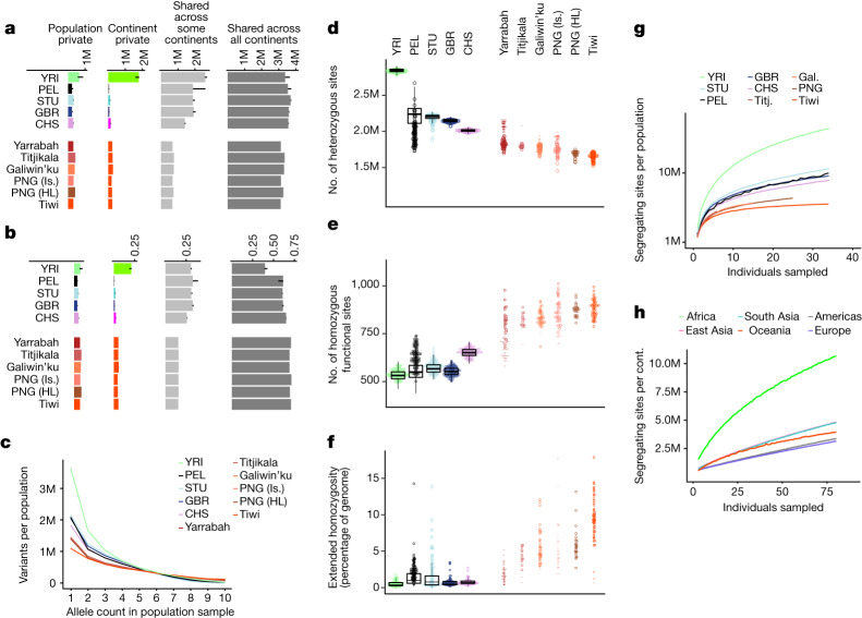
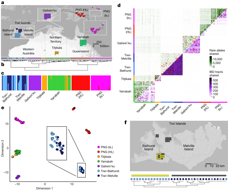
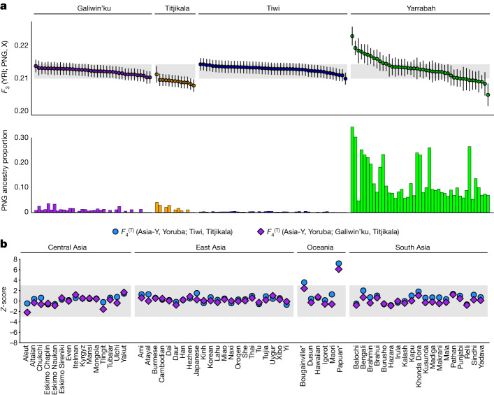
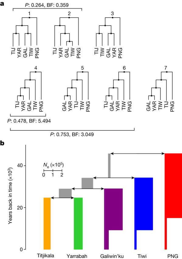
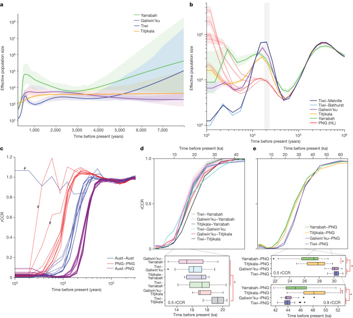
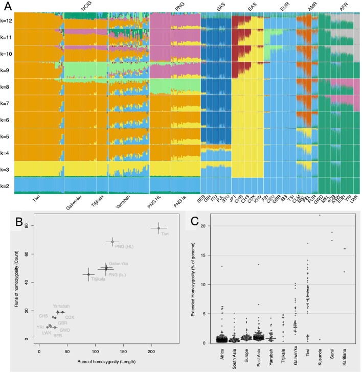
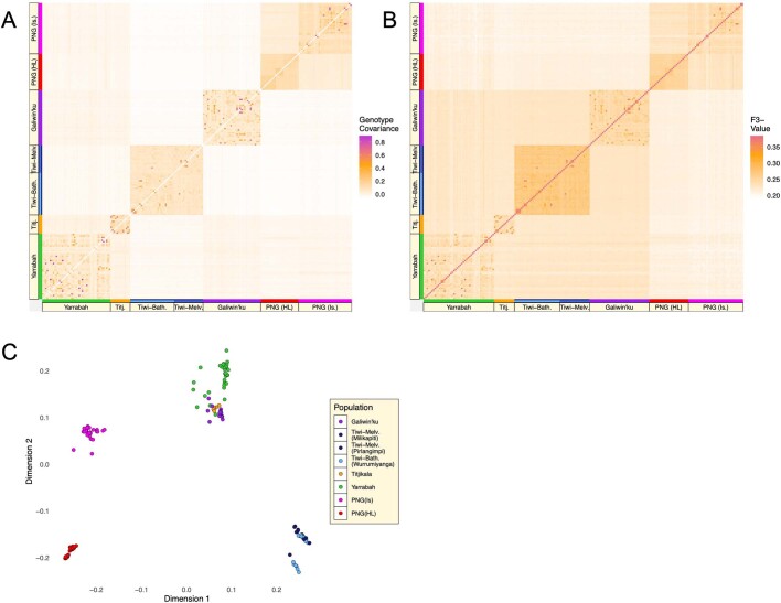
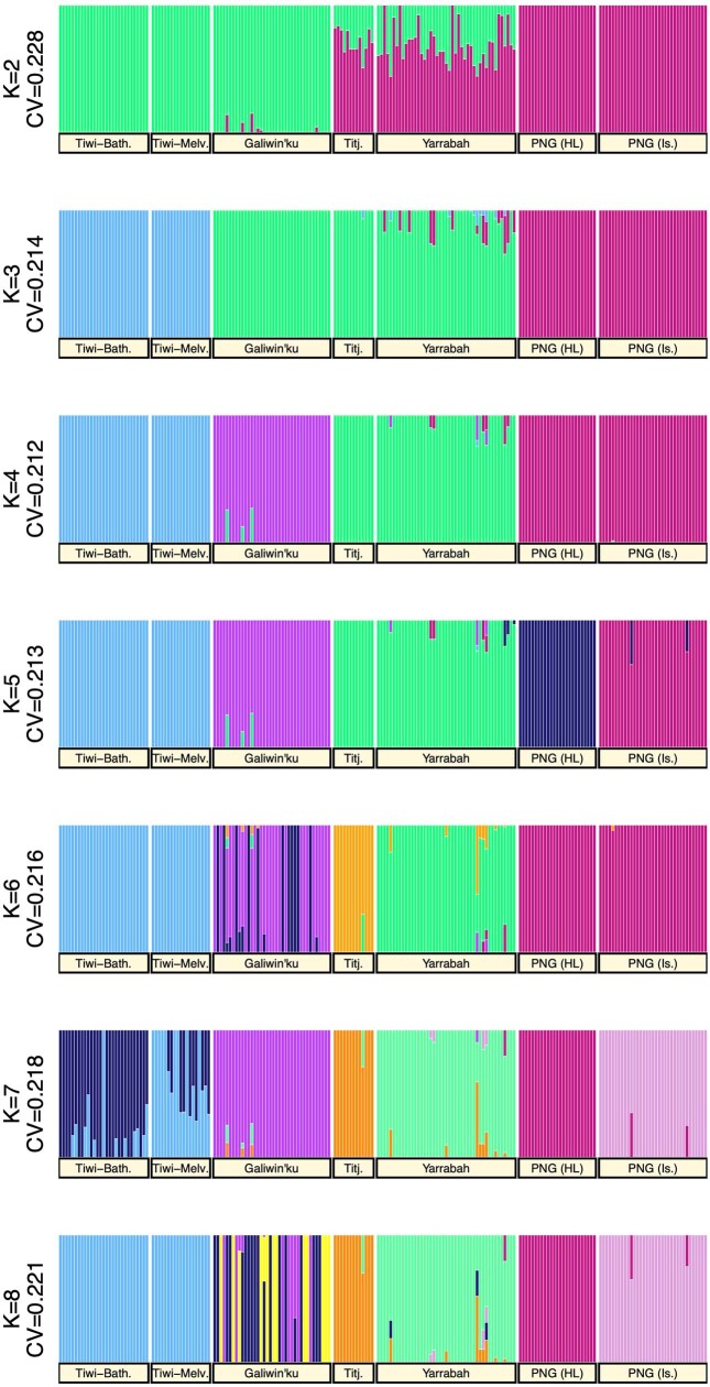
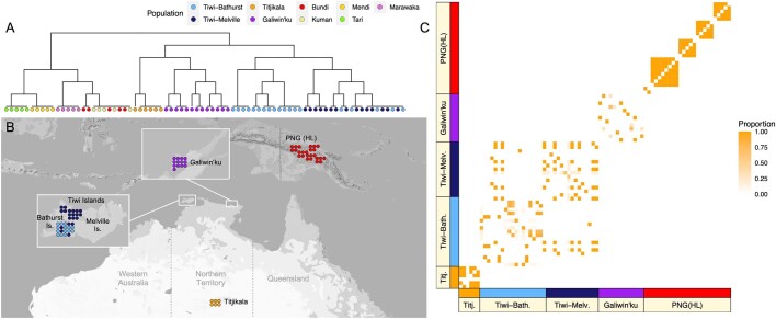
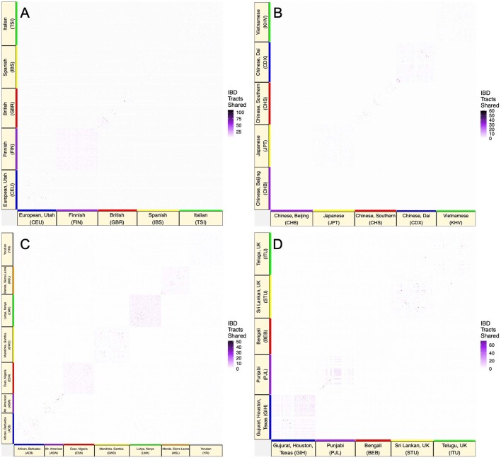
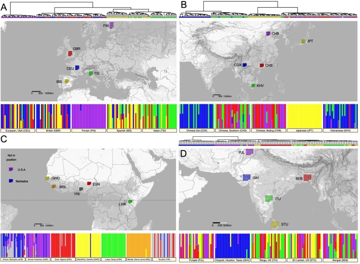
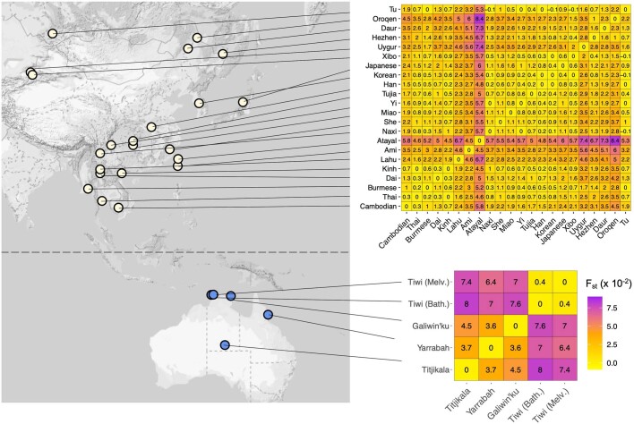
The Indigenous peoples of Australia have a rich linguistic and cultural history. How this relates to genetic diversity remains largely unknown because of their limited engagement with genomic studies. Here we analyse the genomes of 159 individuals from four remote Indigenous communities, including people who speak a language (Tiwi) not from the most widespread family (Pama-Nyungan). This large collection of Indigenous Australian genomes was made possible by careful community engagement and consultation. We observe exceptionally strong population structure across Australia, driven by divergence times between communities of 26,000-35,000 years ago and long-term low but stable effective population sizes. This demographic history, including early divergence from Papua New Guinean (47,000 years ago) and Eurasian groups¹, has generated the highest proportion of previously undescribed genetic variation seen outside Africa and the most extended homozygosity compared with global samples. A substantial proportion of this variation is not observed in global reference panels or clinical datasets, and variation with predicted functional consequence is more likely to be homozygous than in other populations, with consequent implications for medical genomics². Our results show that Indigenous Australians are not a single homogeneous genetic group and their genetic relationship with the peoples of New Guinea is not uniform. These patterns imply that the full breadth of Indigenous Australian genetic diversity remains uncharacterized, potentially limiting genomic medicine and equitable healthcare for Indigenous Australians.

PubMed Disclaimer

Conflict of interest statement

The authors declare no competing interests.

Figures

**Fig. 1. Variant characteristics across populations.**
a,b, Per-population count (a) and proportion of total variation (b) for biallelic SNVs across four classes of sharing for samples of five individuals per population (samples of 15 and 25 in Supplementary Fig. 1). Bars: values for single representative populations. Lines: range for other continental populations. Sharing defined relative to all 26 populations of the 1000 Genomes and the six Oceanic populations considered here. c, Distribution of minor allele count within each population sample (restricted to five as above). Minor allele defined by pooling the five individuals from each of the 32 populations. d–f, Per-individual count of heterozygous sites (d), homozygous amino acid substitutions with predicted functional consequence (e) (SIFT score less than 0.05 (ref. )) and proportion of the genome in extended homozygosity (f) (ROH more than 1 Mb). Outside Oceania, values are for the population indicated, with continental distributions summarized by black box plots (median (line), upper/lower quartiles (box) and 1.5× interquartile range (whiskers)). Values before masking (dashes) and rescaled after masking (circles) are shown for individuals with more than 5% ancestry other than Indigenous ancestry. ROH estimated from unmasked data and therefore not rescaled. ROH values for individuals with more 5% ancestry other than Indigenous ancestry shown as dashes. (Tiwi n = 48, Galiwin’ku n = 38, Titjikala n = 13, Yarrabah n = 45, PNG (HL) n = 25, PNG (Is.) n = 35, YRI n = 108, STU n = 102, GBR n = 91, CHS n = 105, PEL n = 85). g, Variant discovery with increasing sample size per population, averaged (ten replicates). Yarrabah and PNG (Is.) excluded because of missing data after ancestry masking. h, Novel variant discovery per continent after sampling 80 individuals from each of the other continents, averaged (ten replicates). 1000 Genomes codes: YRI, Yoruba, Africa; PEL, Peruvian, America; STU, Sri Lankan, South Asia; GBR, British, Europe; CHS, Southern Han Chinese, East Asia.

**Fig. 2. Population structure.**
a, Location and sample size for all Australian and Papuan samples. b, Hierarchical clustering of unrelated individuals on the basis of pairwise outgroup F₃ statistic values. Colour corresponds to sampling location. c, ADMIXTURE-inferred ancestry for unrelated individuals allowing seven clusters, ordered according to sampling location. Colour was assigned to each cluster post hoc on the basis of the scheme in a and the majority membership of each cluster. d, Pairwise sharing of rare alleles (above diagonal) and IBD (below diagonal) tracts among all individuals. Counts were rescaled according to the proportion of the genome missing due to ancestry masking in each pairwise comparison. Comparisons between first- and second-degree relatives are indicated in red. e, UMAP clustering of unrelated individuals on the basis of minor allele frequency-corrected COV distances, reduced to the first ten components by MDS. Box expands the positions of Tiwi Island individuals. f, Clustering of Tiwi individuals on the basis of co-ancestry values estimated using fineSTRUCTURE run on all unrelated and unadmixed samples (see Extended Data Fig. 4a for the full tree). Light blue (Bathurst Island) and dark blue (Melville Island) indicate sampling location, and yellow and grey indicate cluster membership.

**Fig. 3. Historical relationships between Australian and PNG populations.**
a, Top, shared genetic drift between populations estimated by outgroup F₃ statistics of the form F₃ (Yoruba; PNG, X), where X is an Australian individual. Higher values indicate greater shared genetic drift with PNG. Individuals are rank-ordered by F₃ value within populations, with block jackknife-estimated standard errors shown as vertical bars. The range of F₃ values for individuals in the Tiwi and Galiwin’ku population samples is indicated by horizontal shading. Bottom, the proportion of Papuan global ancestry (after masking) estimated by RFMIX for the same individuals. These per-individual metrics include related individuals. Sample sizes: Tiwi n = 48, Galiwin’ku n = 38, Titjikala n = 13, Yarrabah n = 45. b, Z-scores derived from F₄ statistics of the form $F_{4}^{(T)}$ (Asia-Y, Yoruba; Australia-X, Titjikala), where Asia-Y is a Eurasian or Oceanic population sample from SGDP and Australia-X is either the Galiwin’ku or Tiwi Islands sample. Z-score values greater than 3 provide statistically significant evidence that population Asia-Y shares more genetic drift with Tiwi/Galiwin’ku than with Titjikala, and these populations are marked with an asterisk. The per-individual metrics include related individuals.

**Fig. 4. Historical relationships and processes that have shaped genomic variation in the sample.**
a, Seven plausible population histories were included in ABC simulations, in which effective population sizes and migration rates were allowed to vary. Also shown is the evidence for each scenario or group of scenarios. b, Parameter estimates for split times and effective population sizes for the most likely single scenario, scenario 4 (see Supplementary Figs. 2–4 for parameter distributions). BF, Bayes factor; GAL, Galiwin’ku; N_e, effective population size; P, posterior probability; PNG, Papua New Guinea (HL); TIJ, Titjikala; TIW, Tiwi Islands; YAR, Yarrabah.

**Fig. 5. Effective population sizes and population isolation.**
a, Mean effective population size estimates using the IBDNe algorithm. Shading indicates 95% bootstrap confidence intervals. b, Effective population size estimates for Australian and PNG (HL) populations inferred using MSMC2 from eight phased haplotypes (four individuals) per population. The line and shading are the mean and s.e.m. of five replicates randomly selected from each population sample. Grey bar indicates the Last Glacial Maximum (21 ± 3 ka). c, rCCRs for all 45 possible population pairs (5 Australian + 5 PNG (HL)) estimated with MSMC2. Each line represents the mean rCCR of ten selected sets of eight phased haplotypes (2 haplotypes × 2 individuals × 2 populations). An rCCR of 1 indicates a single ancestral population. An rCCR of 0.5 is a common heuristic indicating the point of population separation. The relative shape of rCCR curves reflects different separation dynamics such as post-split gene flow. Hash indicates three geographically close population pairs (Mendi–Tari, Bundi–Kundiawa in PNG and Bathurst–Melville in Tiwi) that show recent or incomplete separation. d, rCCRs for population pairs within Australia (with Tiwi samples combined), showing mean (line) and s.e.m. (shading) for 10 replicates. Lower box plots show the estimated times of population separation (rCCR = 0.5). Asterisks indicates a significant difference between the Tiwi–Titjikala and all but one of the other separation times. e, rCCRs for population pairs between Australia and PNG (with PNG samples combined) showing mean (line) and s.e.m. (shading) for 10 replicates. Lower box plots show the estimated times of population separation (rCCR = 0.5) and of the onset of population structure (rCCR = 0.9). Asterisks indicate significant differences. All box plots display the median rCCR across 10 replicates (line), upper and lower quartiles (box), 1.5× interquartile range (whiskers) and outliers (points).

**Extended Data Fig. 1. Global ancestry and homozygosity.**
A. Global ancestry proportions for NCIG, Papuan and 1000 Genomes. The software ADMIXTURE run with 159 Indigenous Australian samples, 60 Papuan and 2,600 samples from the LC 1000 Genomes. Samples shown horizontally by population (with reduced bar width for the 1000 Genomes samples) and cluster (colour) assignment proportion shown as bar height. ADMIXTURE was run assuming the sample contained from k = 2 up to k = 12 clusters (y-axis). No ancestry mask applied. Restricted to biallelic SNVs, MAF > 0.01 and LD thinned. This analysis was used to estimate non-Indigenous Australian or PNG ancestry in the NCIG and PNG samples. B. Runs of homozygosity (ROH) for the NCIG + PNG (unmasked) dataset and a subset of (HC) 1000 Genomes samples. Mean count versus mean sum of ROH segments greater than 1 Mb in length. Error bars are within population SEM. Note that a long-term reduction in effective population size is expected to increase both the count and total length of ROH (as seen for NCIG populations), whereas recent consanguinity generates a small number of long ROH. C. Per-individual ROH length (for ROH > 1 Mb) as a percentage of the total autosomal genome length (2.8 Gb). Individuals from three Indigenous populations from Nepal (Kusunda) and Brazil (Surui and Karitiana) from the SGDP were included for comparison as some exhibited extreme levels of ROH. Individuals identified as “Tiwi-outliers” were included in the Tiwi sample in this plot and are evident in panel C as a cluster of individuals with reduced ROH.

**Extended Data Fig. 2. Genetic distances and population structure within Oceania.**
A. Heatmap of the minor allele frequency corrected pairwise covariance (COV) values between all individuals in the NCIG + PNG (masked) dataset (including related individuals). Individuals are listed in the same order along each axis and the population they were sampled from is indicated along the axes. Note that higher values of genotype covariance indicate greater genetic similarity. B. Heatmap of pairwise outgroup F₃-statistics of the form F₃(YRI;AUAx,AUAy), where AUAx and AUAy are any pair of individuals from the NCIG + PNG (masked) dataset (including related individuals). Individuals are listed in the same order along each axis and the population they were sampled from is indicated along the axes. Higher values indicate greater genetic similarity. C. Multidimensional scaling applied to the pairwise genotype covariance (COV) matrix estimated from the *NCIG* + *PNG (masked)* dataset after filtering to unrelated individuals. The first two dimensions are shown. (see Methods for further details of all three plots).

**Extended Data Fig. 3. ADMIXTURE ancestry assignment.**
The clustering algorithm ADMIXTURE applied to the NCIG + PNG (masked) dataset (including related individuals) assuming K = 2 to K = 8 clusters (subpopulations) are represented in the data (See Methods). Clustering makes no reference to the sampling locations of the individuals and is based on genetic data alone. Individuals are listed along the x-axis, grouped according to their sampling location, with bars above reflecting their cluster assignment in the following manner: each inferred cluster is labelled by a colour and the proportion of bar assigned that colour represents the probability that the individual is assigned to that cluster. Colours were manually selected (*post-hoc*) for K = 7 to match the labels in panels 2 A and 2B of Fig. 2, and for other values of K the colouring scheme was merged or split as appropriate. Also shown are the cross-validation (CV) scores used for model selection.

**Extended Data Fig. 4. Fine-scale genetic structure within Oceania.**
A. Hierarchical clustering tree (up to 13 clusters) produced from the maximum *a posteriori* state partitions inferred by fineSTRUCTURE (see Methods). The NCIG + PNG (masked) dataset used for this analysis was reduced to a subset of unadmixed and unrelated samples. Samples are coloured according to their sampling location. Note that the 25 samples from Papua New Guinea are denoted by their sub-sampling locations in this analysis (Bundi, Kundiawa (Kuman), Marawaka, Mendi and Tari). B. Clustering of the NCIG + PNG (masked) dataset into 5 clusters based only on genetic data using fineSTRUCTURE. The dataset used for this analysis was reduced to a subset of unadmixed and unrelated samples. For each individual, the coloured symbol represents the genetic cluster to which the individual is assigned. C. The fineSTRUCTURE coincidence matrix showing the proportion of cluster partitions in which two individuals are grouped in the same cluster during the MCMC. The NCIG + PNG (masked) dataset used for this analysis was reduced to a subset of unadmixed and unrelated samples.

**Extended Data Fig. 5**
**Global IBD tract sharing**. Heatmaps depicting the number of tracts shared IBD (inferred using the RefinedIBD algorithm; see Methods and Supplementary Note 4) within four continental samples from the 1000 Genomes collection: A. Europe, B. East Asia, C. Africa and D. South Asia. A comparable plot featuring NCIG samples is presented in Fig. 2d of the Main Text. Comparisons of samples inferred to share a familial relationship (2nd degree or closer) were masked in red. Note that a different scale was used for each heatmap to maximise definition.

**Extended Data Fig. 6**
**Global population structure**. Results of the ADMIXTURE algorithm and hierarchical clustering of outgroup F₃-statistic values for four continental samples from the 1000 Genomes collection; A. Europe, B. East Asia, C. Africa and D. South Asia. The maps depict the sampling locations for each population, in addition to the sample size used (n = 28 per population). Note that approximate locations for some populations (i.e. CEU, ITU and STU) are given as per the original 1000 Genomes publication. Coloured tip-points below each leaf of the hierarchical clustering tree depict the geographic population label of the individual (from the maps). Hierarchical clustering was not performed on African samples due to the use of Yoruba as the outgroup population (see Methods). The bar charts show the output of the clustering algorithm ADMIXTURE applied to each sample, assuming the same number of clusters as the geographically defined samples (K = 5 for Europe, East Asia and South Asia, and K = 7 for Africa). Clustering makes no reference to the sampling locations of the individuals and is based on genetic data alone. Individuals are listed along the x-axis, grouped according to their sampling location, with bars above reflecting their cluster assignment in the following manner: each inferred cluster is labelled by a colour and the proportion of bar assigned that colour represents the probability that the individual is assigned to that cluster. Colours were manually selected (post-hoc) to match the labels in the maps. See Fig. 2 of the main text for the results of these same algorithms when applied to the NCIG + PNG dataset.

**Extended Data Fig. 7. Pairwise F_ST between Australian, PNG and Asian populations from the SGDP.**
Genetic differences between Indigenous Australian communities are significantly greater than between groups from other continents distributed over a comparable geographic range. Heatmaps show pairwise F_ST differences between all East Asian populations, and all Australian communities. Note, for instance, F_ST between Galiwin’ku and Titjikala (0.045), is as high as between Cambodia and Oroqen (0.045), groups separated by three to four times the geographical distance. All F_ST values were calculated on a set of variants polymorphic in an African outgroup population (Mbuti), thus providing an unbiased estimator of F_ST. Colour scales for both heatmaps are the same.

**Extended Data Fig. 8. Comparing genetic drift shared with PNG using F-statistics.**
A. p-values from a Mann Whitney U test performed pairwise between the Australian samples grouped by community. Here we assume that the outgroup F₃ statistic for each individual (relative to PNG) in Fig. 3a is drawn from a common distribution for each community. The distributions of the statistic for a pair of communities are compared using the Mann Whitney test. Significant p-values (less than 0.05; shown in red) indicate the null hypothesis, that the distributions of the statistic for each group are equal, has been rejected. A two-sided test was used, with the Bonferroni p-value adjustment method. B. Matrix of all pairwise $F_{4}^{(T)}$ statistics (calculated using ADMIXTOOLS) of the form $F_{4}^{(T)}$ (YRI, PNG; X, Y), where ‘X’ and ‘Y’ are any one of the Australian populations in the NCIG dataset. Here we separate the Tiwi samples into the islands they are sampled from. Numbers reported are Z scores (the default ADMIXTOOLS output) and are significant when they exceed +3 or −3. See Methods for description of ‘Tiwi_Outlier’ label. C. Table showing all possible F₃ statistics of the form F₃(AUAx; PNG, AUAy), where ‘AUAx’ and ‘AUAy’ (simply labelled ‘X’ and ‘Y’ in this figure) are a pair of groups from the NCIG dataset. Here we separate the Tiwi samples into the two islands, Bathurst and Melville, and we also treat the Tiwi Outlier individuals as a separate group (See Methods for a description of the Tiwi Outlier individuals and a justification for removing them from our main analyses due to evidence of substantial recent admixture with PNG in their genomes). Text within each cell is the Z-score for the F₃ statistic from a block jackknife (directly from the software Admixtools). Following the theory of Patterson et al. (2012), statistically significant evidence of admixture between PNG and AUAx, but not AUAy, is indicated by a Z-score lower than −3, here indicated by red.

**Extended Data Fig. 9. Shared genetic drift between Indigenous Australian communities and a panel of Papuan populations.**
(Left) Map showing the locations of all populations sampled in the dataset of Bergstrom et al. (2017), with colour code indicating the regional province. (Top Right) Scatterplot of values of outgroup F₃ statistics of the form F₃(Yoruba; Titjikala, PNG-X) versus F₃(Yoruba; Tiwi, PNG-X), where ‘PNG-X’ is a PNG individual in the dataset described by Bergstrom et al. (2017). Colours represent the sampling location of the PNG individual (see map to the left). (Bottom Right) ADMIXTURE barplot showing putative PNG (yellow) and non-PNG (purple) global ancestry estimates for each of the individuals in the above scatterplot. Individuals in the barplot are shown in the same order left to right as in the scatterplot.

**Extended Data Fig. 10**
**Mitochondrial phylogenetics**. Population Mitochondrial DNA phylogeny of all individuals from the ***NCIG*** + ***PNG*** dataset, plus additional sequences from GenBank (see Methods and Supplementary Note 7 for samples used and phylogenetic methods). Tip-point labels indicate the community the individual was sampled from. Coloured circles over nodes indicate coalescence events between PNG and Indigenous Australian haplotypes which date to within the last ~35 ka. Clade labels of sub-lineages (P3, N13 and Q2) mark the lineages involved.

**Extended Data Fig. 11. Map with pie charts showing frequencies of the P3, N13 and Q2 Mitochondrial haplogroups.**
Map with pie charts showing frequencies of the three haplogroups (P3, N13 and Q2), with recent (~35 ka) TMRCA to Melanesian sister lineages in Indigenous Australian communities from both the NCIG dataset, and previously published studies. Note the apparent enrichment of these haplogroups in the Top End and Kimberley regions of Australia. The P3 haplogroup frequency was scored instead of P3b, as some studies did not genotype to this degree of resolution. The P3 lineage coalesces approximately 35 ka and contains both PNG and Indigenous Australian sub-lineages.

See this image and copyright information in PMC

Cited by

Precision medicine in Australia: indigenous health professionals are needed to improve equity for Aboriginal and Torres Strait Islanders.
Lewis DA, Mitchell T, Kowal E. Lewis DA, et al. Int J Equity Health. 2024 Jul 4;23(1):134. doi: 10.1186/s12939-024-02202-7. Int J Equity Health. 2024. PMID: 38965527 Free PMC article.
Australian Indigenous genomes are highly diverse and unlike those anywhere else.
Nogrady B. Nogrady B. Nature. 2024 Jan;625(7993):15-16. doi: 10.1038/d41586-023-04006-1. Nature. 2024. PMID: 38093071 No abstract available.
Increasing Diversity, Equity, Inclusion, and Accessibility in Rare Disease Clinical Trials.
Baynam G, Baker S, Steward C, Summar M, Halley M, Pariser A. Baynam G, et al. Pharmaceut Med. 2024 Jul;38(4):261-276. doi: 10.1007/s40290-024-00529-8. Epub 2024 Jul 9. Pharmaceut Med. 2024. PMID: 38977611 Review.
A call to action to scale up research and clinical genomic data sharing.
Stark Z, Glazer D, Hofmann O, Rendon A, Marshall CR, Ginsburg GS, Lunt C, Allen N, Effingham M, Hastings Ward J, Hill SL, Ali R, Goodhand P, Page A, Rehm HL, North KN, Scott RH. Stark Z, et al. Nat Rev Genet. 2025 Feb;26(2):141-147. doi: 10.1038/s41576-024-00776-0. Epub 2024 Oct 7. Nat Rev Genet. 2025. PMID: 39375561 Review.
Estimating evolutionary and demographic parameters via ARG-derived IBD.
Huang Z, Kelleher J, Chan YB, Balding DJ. Huang Z, et al. bioRxiv [Preprint]. 2024 Mar 13:2024.03.07.583855. doi: 10.1101/2024.03.07.583855. bioRxiv. 2024. Update in: PLoS Genet. 2025 Jan 8;21(1):e1011537. doi: 10.1371/journal.pgen.1011537. PMID: 38559261 Free PMC article. Updated. Preprint.

References

1. Malaspinas AS, et al. A genomic history of Aboriginal Australia. Nature. 2016;538:207–214. doi: 10.1038/nature18299. - DOI - PubMed
1. Henn BM, et al. Distance from sub-Saharan Africa predicts mutational load in diverse human genomes. Proc. Natl Acad. Sci. USA. 2016;113:E440–E449. doi: 10.1073/pnas.1510805112. - DOI - PMC - PubMed
1. Rasmussen M, et al. An Aboriginal Australian genome reveals separate human dispersals into Asia. Science. 2011;334:94–98. doi: 10.1126/science.1211177. - DOI - PMC - PubMed
1. Jacobs GS, et al. Multiple deeply divergent denisovan ancestries in Papuans. Cell. 2019;177:1010–1021.e32. doi: 10.1016/j.cell.2019.02.035. - DOI - PubMed
1. Vernot B, et al. Excavating Neandertal and Denisovan DNA from the genomes of Melanesian individuals. Science. 2016;352:235–239. doi: 10.1126/science.aad9416. - DOI - PMC - PubMed

MeSH terms

Actions
Actions
Actions
Actions
Actions
Actions
Actions
Actions
Actions
Actions
Actions
Actions
Actions
Actions
Actions
Actions

Supplementary concepts

Actions

LinkOut - more resources

Full Text Sources

[1] Malaspinas AS, et al. A genomic history of Aboriginal Australia. Nature. 2016;538:207–214. doi: 10.1038/nature18299. - DOI - PubMed

[2] Malaspinas AS, et al. A genomic history of Aboriginal Australia. Nature. 2016;538:207–214. doi: 10.1038/nature18299. - DOI - PubMed

[3] Henn BM, et al. Distance from sub-Saharan Africa predicts mutational load in diverse human genomes. Proc. Natl Acad. Sci. USA. 2016;113:E440–E449. doi: 10.1073/pnas.1510805112. - DOI - PMC - PubMed

[4] Henn BM, et al. Distance from sub-Saharan Africa predicts mutational load in diverse human genomes. Proc. Natl Acad. Sci. USA. 2016;113:E440–E449. doi: 10.1073/pnas.1510805112. - DOI - PMC - PubMed

[5] Rasmussen M, et al. An Aboriginal Australian genome reveals separate human dispersals into Asia. Science. 2011;334:94–98. doi: 10.1126/science.1211177. - DOI - PMC - PubMed

[6] Rasmussen M, et al. An Aboriginal Australian genome reveals separate human dispersals into Asia. Science. 2011;334:94–98. doi: 10.1126/science.1211177. - DOI - PMC - PubMed

[7] Jacobs GS, et al. Multiple deeply divergent denisovan ancestries in Papuans. Cell. 2019;177:1010–1021.e32. doi: 10.1016/j.cell.2019.02.035. - DOI - PubMed

[8] Jacobs GS, et al. Multiple deeply divergent denisovan ancestries in Papuans. Cell. 2019;177:1010–1021.e32. doi: 10.1016/j.cell.2019.02.035. - DOI - PubMed

[9] Vernot B, et al. Excavating Neandertal and Denisovan DNA from the genomes of Melanesian individuals. Science. 2016;352:235–239. doi: 10.1126/science.aad9416. - DOI - PMC - PubMed

[10] Vernot B, et al. Excavating Neandertal and Denisovan DNA from the genomes of Melanesian individuals. Science. 2016;352:235–239. doi: 10.1126/science.aad9416. - DOI - PMC - PubMed

Save citation to file

Email citation

Add to Collections

Add to My Bibliography

Your saved search

Create a file for external citation management software

Your RSS Feed

Indigenous Australian genomes show deep structure and rich novel variation

Collaborators

Affiliations

Indigenous Australian genomes show deep structure and rich novel variation

Authors

Collaborators

Affiliations

Abstract

Conflict of interest statement

Figures

Similar articles

Cited by

References

MeSH terms

Supplementary concepts

LinkOut - more resources

Full Text Sources

Abstract

Conflict of interest statement

Figures

Similar articles

Cited by

References

MeSH terms

Supplementary concepts

Related information

LinkOut - more resources

Full Text Sources